
I figured out how to engineer emergence
The results from my return to science

“Look to the rock from which you were hewn” — Isaiah 51:1
Earlier this year I returned to science because I had a dream.
I had a dream where I could see inside a system’s workings, and inside were what looked like weathered rock faces with differing topographies. They reminded me of rock formations you might see in the desert: some were “ventifacts,” top-heavy structures carved by the wind and rain, while others were bottom-heavy, like pyramids; there were those that bulged fatly around the middle, or ones that stood straight up like thin poles.

Consider this an oneiric announcement: almost a year later, I’ve now published a paper, “Engineering Emergence,” that renders this dream flesh. Or renders it math, at least.
But back when I had the dream I hadn’t published a science paper in almost two years. I had, however, been dwelling on an idea.
A little backstory: in 2013 my co-authors and I introduced a mathematical theory of emergence focused on causation (eponymously dubbed “causal emergence”). The theory was unusual, because it viewed emergence as a common, everyday phenomenon, occurring despite how a system’s higher levels (called “macroscales”) were still firmly reducible to their microscales.
The theory pointed out that causal relationships up at the macroscale have an innate advantage: they are less affected by noise and uncertainty. Conditional probabilities (the chances governing statements like if X then Y) can be much stronger between macro-variables than micro-variables, even when they’re just two alternative levels of description of the very same thing.
How is that possible? I posited it’s because of what in information theory is called “error correction.” Essentially, macroscale causal relationships take advantage of the one thing that can never be reduced to their underlying microscale: they are what philosophers call “multiply realizable” (e.g., the macro-variable of temperature encapsulates many possible configurations of particles). And the theory of causal emergence points out this means they can correct errors in causal relationships in ways their microscale cannot.
The theory has grown into a bit of a cult classic of research. It’s collected hundreds of citations and been applied to a number of empirical studies; there are scientific reviews of causal-emergence-related literature, and the theory has been featured in several books, such as Philip Ball’s How Life Works.
However, it never became truly popular, and also—probably relatedly—it never felt complete to me.
One thing in particular bothered me: in our original formulation (with co-authors Giulio Tononi and Larissa Albantakis) we designed the theory to identify just a single emergent macroscale of interest.1
But don’t systems have many viable scales of description, not just one?
You can describe a computer down at the microscale of its physical logic gates, in the middle mesoscale of its machine code, or up at the macroscale of its operating system. You can describe the brain as a massive set of molecular machinery ticking away, but also as a bunch of neurons and their input-output signals, or even as the dynamics of a group of interconnected cortical minicolumns or entire brain regions, not to mention also at the level of your psychology. And all these seem, at least potentially, like valid descriptions.
It’s as if inside any complex system is a hierarchy, a structure that spans spatiotemporal scales, containing lots of hidden structure.2 Thus, the dreamland of rock formations with their different shapes.

It turns out this portentous dream was quite real, and we now finally have the math to reveal these structures.
This new paper also completes a new and improved “Causal Emergence 2.0” that keeps a lot of what worked from the original theory a decade ago but also departs from it in several key ways (including negating older criticisms), especially around multiscale structure. It makes me feel that I’ve finally done the old idea justice, given its promise.
This latest paper on Causal Emergence 2.0 was co-authored by Abel Jansma and myself. Abel is an amazingly creative researcher, and also a great collaborator (you can find his blog here). Here’s our title and abstract:
One of our coolest results is that we figured out ways to engineer causal emergence, to grow it and shape it.
And, God help us all, I’m going to try to explain how we did that.

For any given system, you’ll be able to—
Hold on. Just wait a second. You keep using that word, “system.” It’s an abstract blob to me. What should I actually envision?
That’s a great place to start! The etymology of the word “system” is something like “I cause to stand together.”
My meaning here is close to its roots: by “system” I mean a thing or process that can be described as an abstract succession of states. Basically, anything that is in some current state and then moves to the next state.
Lots of things can be represented this way. Let’s say you were playing a game of Snakes and Ladders. Your current board state is just the number: 1…100. So the game has exactly 100 states.

At any given state, the transition to the next state is entirely determined by a die roll. You can think of this as each state having a probability of transition, p. And we know that p = 1/6 over some set of next 6 possible states. In this, Snakes and Ladders forms a massive “absorbing” Markov chain, where eventually, if you roll enough dice, you always reach the end of the game. Being a “Markov chain” is just a fancy way of saying that the current state solely determines the next state (it doesn’t matter where you were three moves ago, what matters is where your figurine is now on the board). In this, Snakes and Ladders is secretly a machine that ticks away from state to state as it operates; thus, Markov chains are sometimes called “state machines.”
Lots of board games can be represented as Markov chains. So can gene regulatory networks, which are critically important in biology. If you believe Stephen Wolfram, the entire universe is basically just a big state machine, ticking away. Regardless, it’s enough for our purposes (defining and showcasing the theory) that many systems in science can be described in this way.
Now, imagine you are given a nameless system, i.e., some Markov chain. And you don’t know what it represents (it could be a new version of Snakes and Ladders, or a gene regulatory network, or a network of logic gates, or tiny interacting discrete particles). But you do know, a priori, that it’s fully accurate, in that it contains every state, and also it precisely describes their probability of transitioning. Imagine it’s this one:
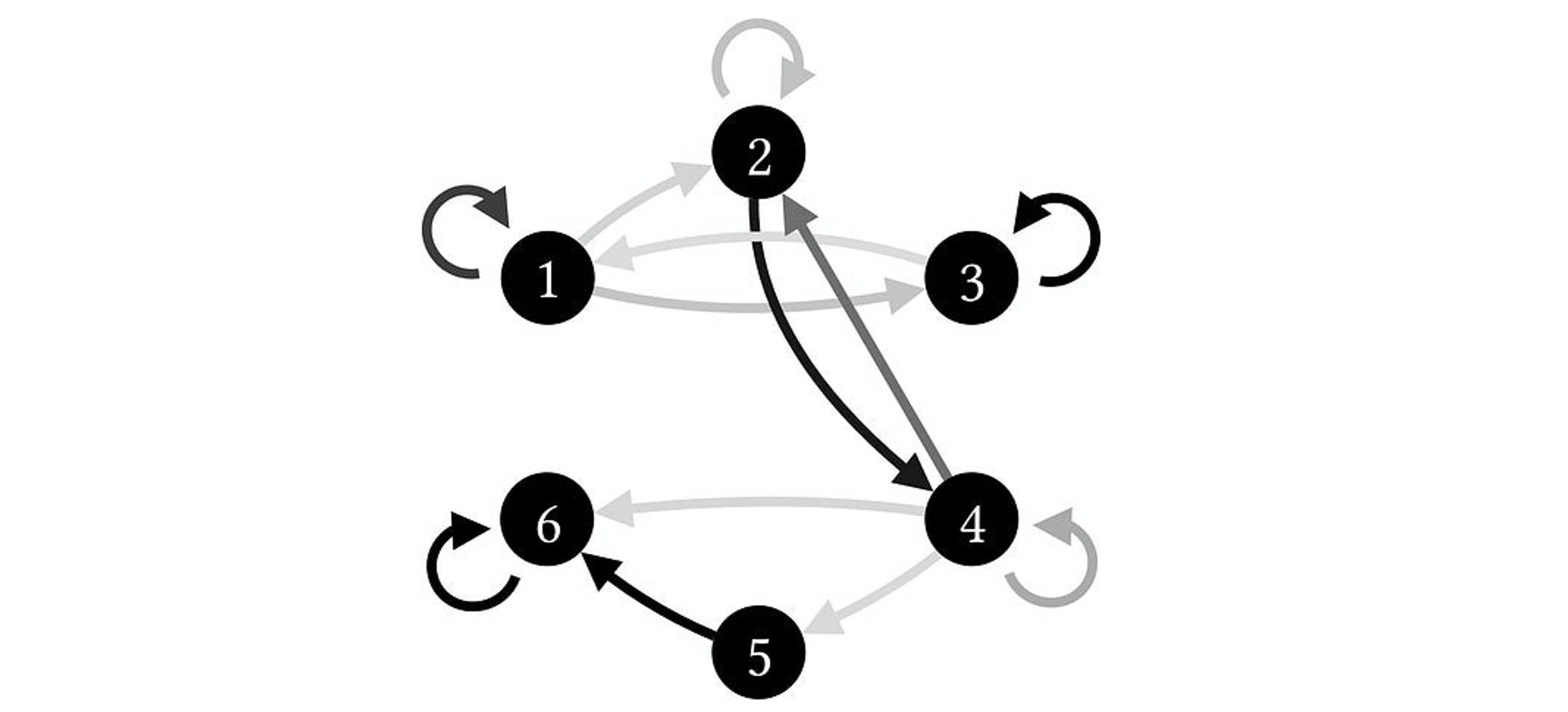
This system has 6 states. You can call them states “1” or “2,” or you could label them things like “A” or “B.” The probabilities of transitioning from one state to the next are represented by arrows in grayscale. I’m not telling you what those probabilities are because those details don’t matter. What matters is that if an arrow is black, it reflects a high probability of transitioning (p = ~1). The lighter the arrows are, the less likely that transition is. So the 1 → 1 transition is more likely than the 1 → 2 transition.
You can also represent this as a network of states or as a Transition Probability Matrix (TPM), wherein each row tells the probabilities of what will happen if the system is in a particular state at time t. For the system above, its TPM would look like this:

Again, the probabilities are grayscale, with black being p = ~1. But you can confirm this is the same thing as the network visualization of the states above; e.g., state 6 will transition to state 6 with p = 1 (the entry on the bottom right), which is the same as the self-loop above.
Each state can also be conceived of as possible cause or a possible effect. For instance, state 5 can cause state 6 (specified by the black entry in the TPM just above the furthest to the bottom right). You can imagine a little man hopping from one state to another state to represent the system’s causal workings (“What does what?” as it ticks away).
Causation is different from mere observation. To really understand causation, we must intervene. For instance, let’s say the system is sitting in state 6. From observations alone we might think that only state 6 is the cause of state 6 (the self-loop). However, we can intervene directly to verify. Imagine here that we “reach into” the system and set it to a state. This would be like moving our figurine in Snakes and Ladders to a particular place on the board via deus ex machina.
This is sometimes described formally with a “do-operator,” and can written in shorthand as do(5), which would imply moving the system to state 5 (irrespective of what was happening before). If we intervene to “do” state 5, we then immediately see that state 6 is not actually the sole cause of state 6, but state 5 is too, and therefore we know that state 6 is not necessary for producing state 6. It reveals the causal relationship via a counterfactual analysis: “If the system had not been in state 6, what could it have been instead and achieved the same effect?” and the answer is “state 5.”
Ok, I get it. By “system” you mean an abstract machine made of states. And the states can have causal relationships.
Great! But I regret to inform you that each system contains within it other systems. Many, many, many other systems. Or at least, other ways to look at the system that change its nature. We call these “scales of description,” and even for small systems there are a lot of them (technically, the Bell number of its n states). It’s like every system is really a high-dimensional object, and individual scales are just low-dimensional slices.
The many scales of description can themselves be represented by a huge set of partitions. For a system with 3 states, these partitions might be (12)(3) or (1)(2)(3) or (123).
What does a partition like (12)(3) actually mean? Basically, something like: “we consider (12) to be grouped together, but (3) is still its own thing.” A partition wherein everything is grouped into one big chunk, like (123), is an ultimate macroscale. A partition where nothing is grouped together, consisting of separate chunks the exact size of the individual original states, like (1)(2)(3), is a microscale. Here’s every possible partition of a system with a measly five states.

That’s a lot of scales! How do we wrangle this into a coherent multiscale structure?
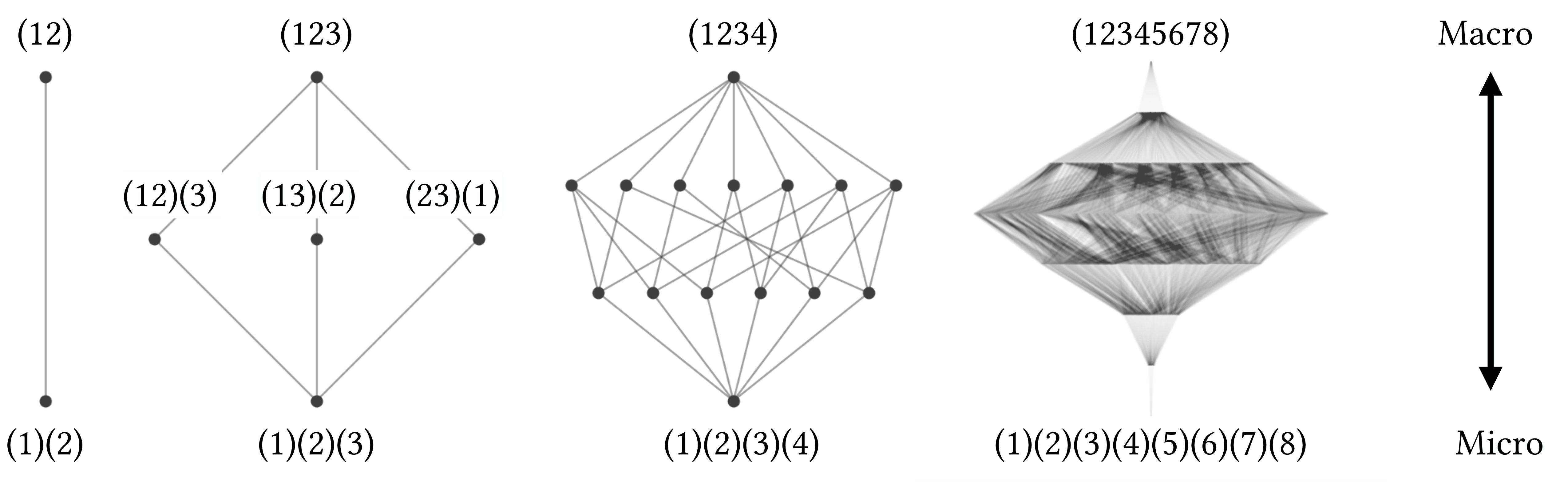
Mathematically, we can order this set of partitions into a big lattice. Here, a “lattice” is basically just another fancy term for a structure ordered by refinement, as in partitions of the same size (the same “chunkiness”) all in a row together. The ultimate macroscale is at the top, the microscale is at the bottom, and partitions get “chunkier” (more coarse-grained) as you go up. This is the beginning of how we think about multiscale structure.
Here are some different lattices of systems of varying sizes, ranging from just 2 states (left) all the way to 8 states (right).
However, even the lattices don’t give us the entire multiscale structure. They give us a bunch of “group this together” directions. These directions can be turned into actual scales, by which we mean other TPMs that operate like the microscale one, but are smaller (since things have been grouped together).
So TPMs spawn other TPMs? Even small and simple ones?
Exactly. Not to get too biblical, but the microscale is the wellspring from which the multiscale structure emerges.
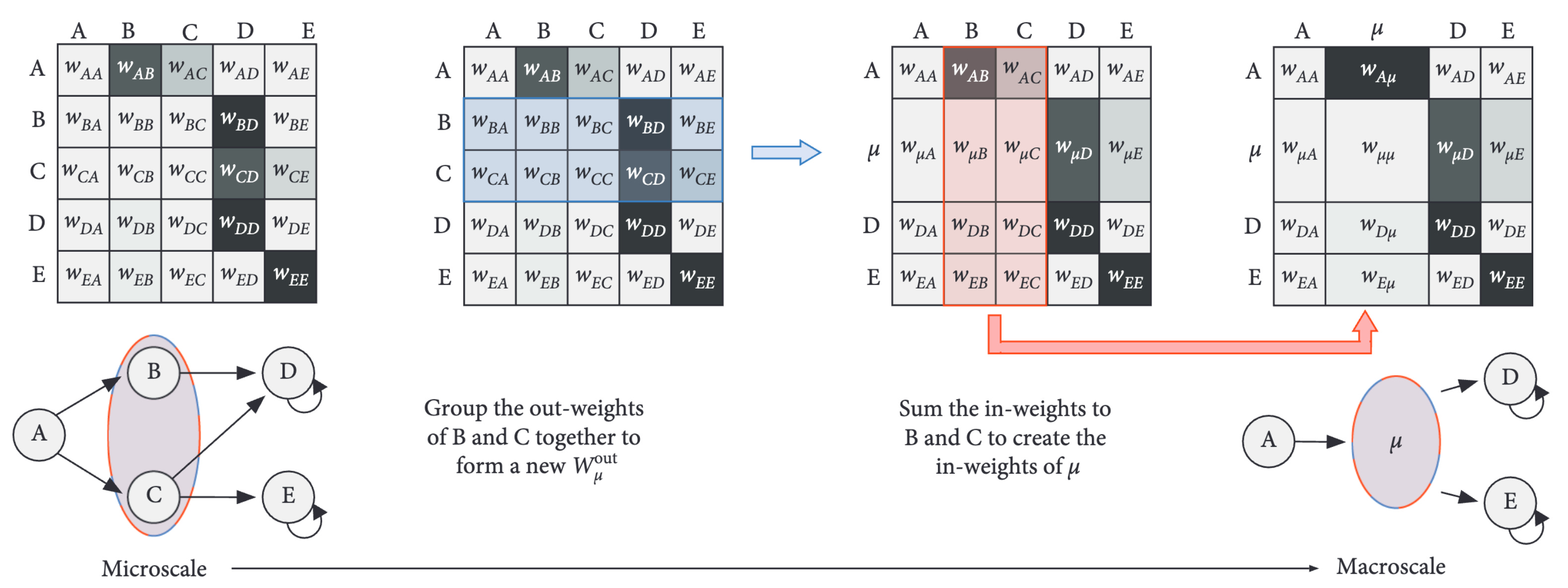
To identify all the TPMs at higher scales, operationally we kind of just squish the microscale TPM into different TPMs with fewer rows and columns, according to some partition (and do this for all partitions). This squishing is shown below. Importantly, this can be done cleverly in such a way that both dynamics and the effects of interventions are preserved. E.g., if you were to put the system visualized as a Markov chain below in state A (as in do(A)), the same series of events would unfold at both the microscale TPM and the shown macroscale TPM (e.g., given A, the system ends up at D or E after two timesteps, with identical probabilities).
But it should be intuitively obvious that some squishings are superior to others.
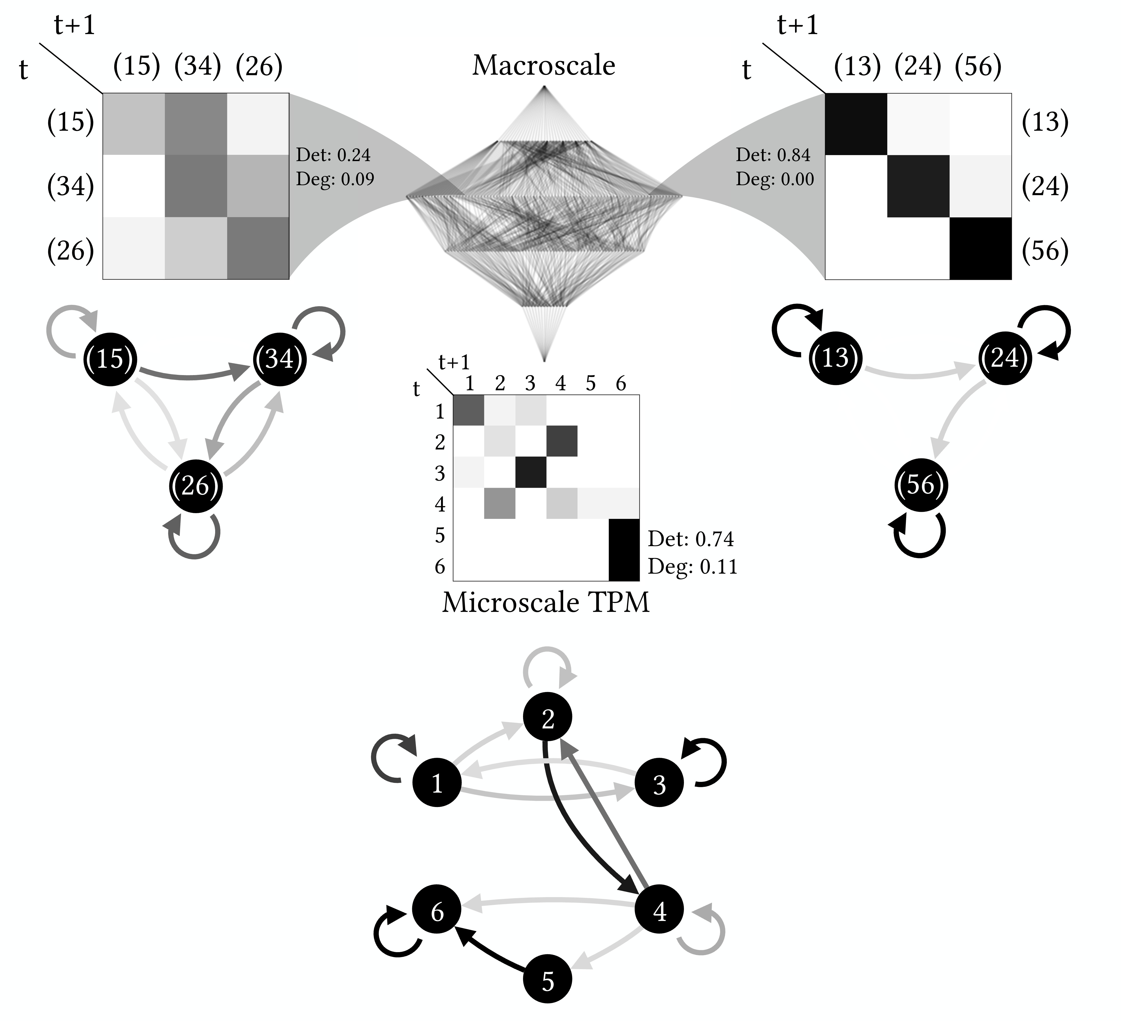
Below is an example from our trusty 6-state system. The 6-state system acts as the original “wellspring” microscale TPM, with its visualization as a state machine at the bottom, and its lattice of partitions is in the middle. Also shown are two different scales taken from the same level (the same chunkiness, i.e., from the same row in the lattice of partitions), each with a squished macroscale TPM (seen on the left and right). Again, probabilities are in grayscale. But one macroscale TPM is junk (left), while the other is not (right).
Hmmm, but “junk” seems subjective.
It is. For now.
One job of a theory is to translate subjective judgements like “good” and “bad” into something more formal. The root of the “junk” judgement is because the macroscale TPM is noisy. Luckily, it’s possible to explicitly formalize how much each scale contributes to the system’s causal workings, which is also sensitive to this “noisiness,” and put a number, or score, on each possible scale and its TPM.
Specifically, for each scale’s TPM, we calculate its determinism and its degeneracy. The actual math to calculate these terms is not that complicated,3 if you already know some information theory, like what entropy is. The determinism is based on the entropy of the effects (future states) given a particular cause (current state):

And the degeneracy is based on the entropy of the effects overall:

Wait! What if I don’t know what the entropy is?!
Totally fine. Just think of it like this: these terms are like a TPM’s score that reflects its causal contribution. Determinism would be maximal (i.e., = 1) if there were just a lone p = 1 in a row (a single entry, with the rest p = 0). And its determinism would be minimal if the row was entirely filled with entries of p = 1/n, where n is the length of the row (i.e., the probabilities are completely smeared out). The entropy is just a smooth way to track the difference between that maximal and minimal situation (are the probabilities concentrated, and so close to 1, or smeared out?).
The degeneracy is trickier to understand but, in principle, quite similar. Degeneracy would be maximal (= 1) if all the states deterministically led to just one state (i.e., all causes always had the same effect in the system). If every cause led deterministically to a unique effect (each cause has a different effect), then degeneracy would be 0.
The determinism and degeneracy are kind of like information-theoretic fancy ways of capturing the sufficiency and necessity of the causal relationships between the states (although the necessity would be more so the reverse of the degeneracy). If I were to look at a system and say “Hey, its causal relationships have high sufficiency and necessity!” I could also say something like “Hey, its causal relationships have high determinism and low degeneracy!” or I could say “Hey, its probabilities of transitions between states are concentrated in different regions of its state-space and not smeared or overlapping” and I would be saying pretty much the same thing in each case.
Using these terms, the updated theory (Causal Emergence 2.0) formalizes a score for a TPM that ranges from 0 to 1. Mathematically, the score is basically just the determinism and degeneracy combined together (but remember, the degeneracy must be inverted). You can think of the score as the causal contribution by the TPM to the overall system’s workings (or as the causal relationships of that TPM having a certain power, or strength, or constraint, or informativeness—there are a ton of synonyms for “causal contribution”).
So every scale has some causal contribution? Doesn’t that mean they all contribute to the system’s causal workings?
Yes! And no. That’s what Abel and I figured out in this new paper.
Basically, the situation leads to an embarrassment of multiplicity. Either you say everything is overdetermined, or you say that only the microscale is really doing anything (the classic reductionist option). Both of these have the problem of being absurd. One is a zany relativism that treats all scales the same and ignores their ordered structure as a hierarchy, while the other is a hardcore reductionism implying that all causation “drains away” to the bottom microscale (to use a phrase from philosopher Ned Block), rendering the majority of the elements of science (and daily life) epiphenomenal.
Instead, we present a third, much more sensible option: macroscales can causally contribute, but only if they add to the causal workings in a manner that’s not reducible compared to the microscale, or any other scale “beneath them.” We can apportion out the causation, as if we were cutting up a pie fairly. We can look at every point on the lattice and ask: “Does this actually add causal contributions that are irreducible?”
For most scales, the answer to this question is “No.” As in, what they are contributing the system’s causal workings is reducible. However, a small subset are irreducible in their contributions.
The figure below shows the process to find all these actually causally contributing scales for a given TPM (shown tiny at the very bottom). In panel A (on the left) we see the full lattice, and, within it, the meager 4 scales (beyond the microscale) that irreducibly causally contribute, after a thorough check of every scale on the path below them.
In the middle (B) you can see the actually causally-contributing scales plotted by themselves, wherein the size of the black dot is their overall relative contribution. This is an emergent hierarchy: it is emergent because all members are scales above the microscale that have positive causal contributions when checked against every scale below it, and it is a hierarchy because they can still be ordered from finest (the microscale) up to the coarsest (the “biggest” macroscale).
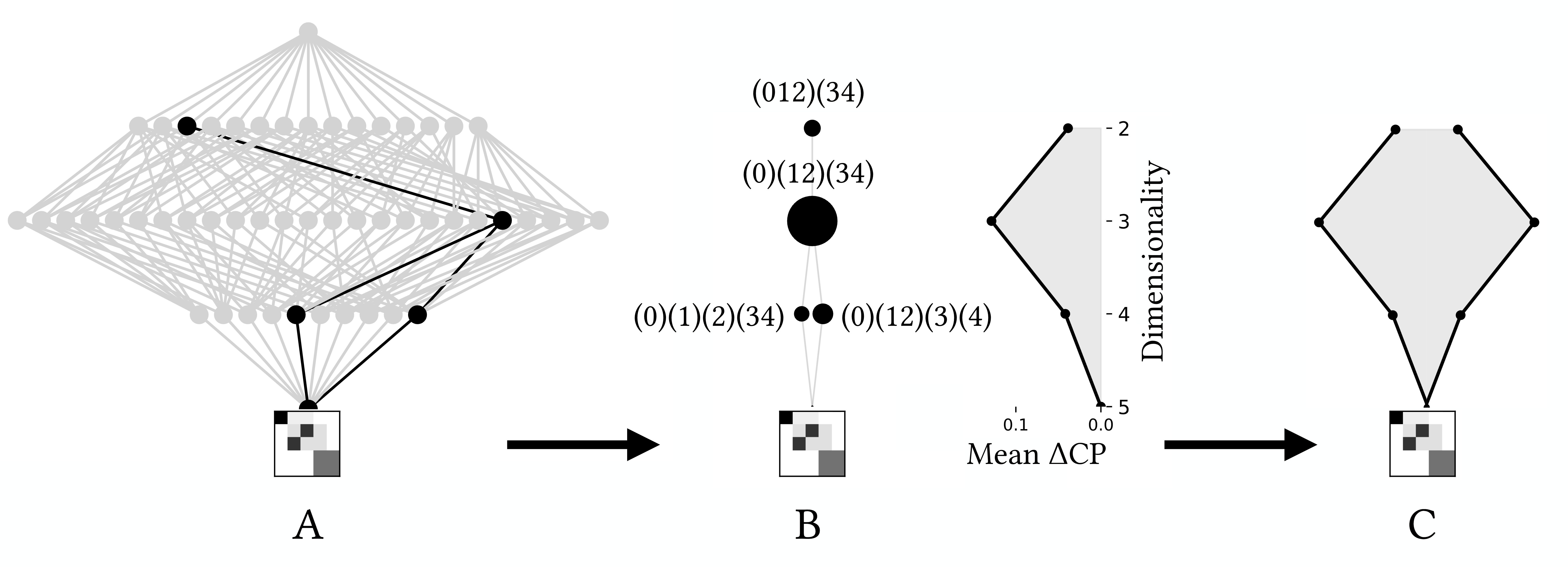
We can chart the average irreducible causal contribution at each level (listed as Mean ΔCP, because sometimes the determinism/degeneracy are called “causal primitives”) and get a sense of how the contributions are distributed across the levels of the system. For this system, most of the irreducible contribution is gained at the mesoscale, that is, a middle-ish level of a system (where the big black dot is). A further visualization of this distribution is shown in (C), on the far right, which is just a mirrored and expanded version of the distribution on its left so that the shape is visible.
These hidden emergent hierarchies can be of many different types. Abel and I put together a little “rock garden” of them in the figure below. You can see the TPMs of the microscale at the bottoms, with the resultant emergent hierarchy “growing” out of it above. Below each is plotted the overall average causal contribution distribution across the scales. Causally, some systems are quite “top-heavy,” while others are more “bottom-heavy,” and so on.
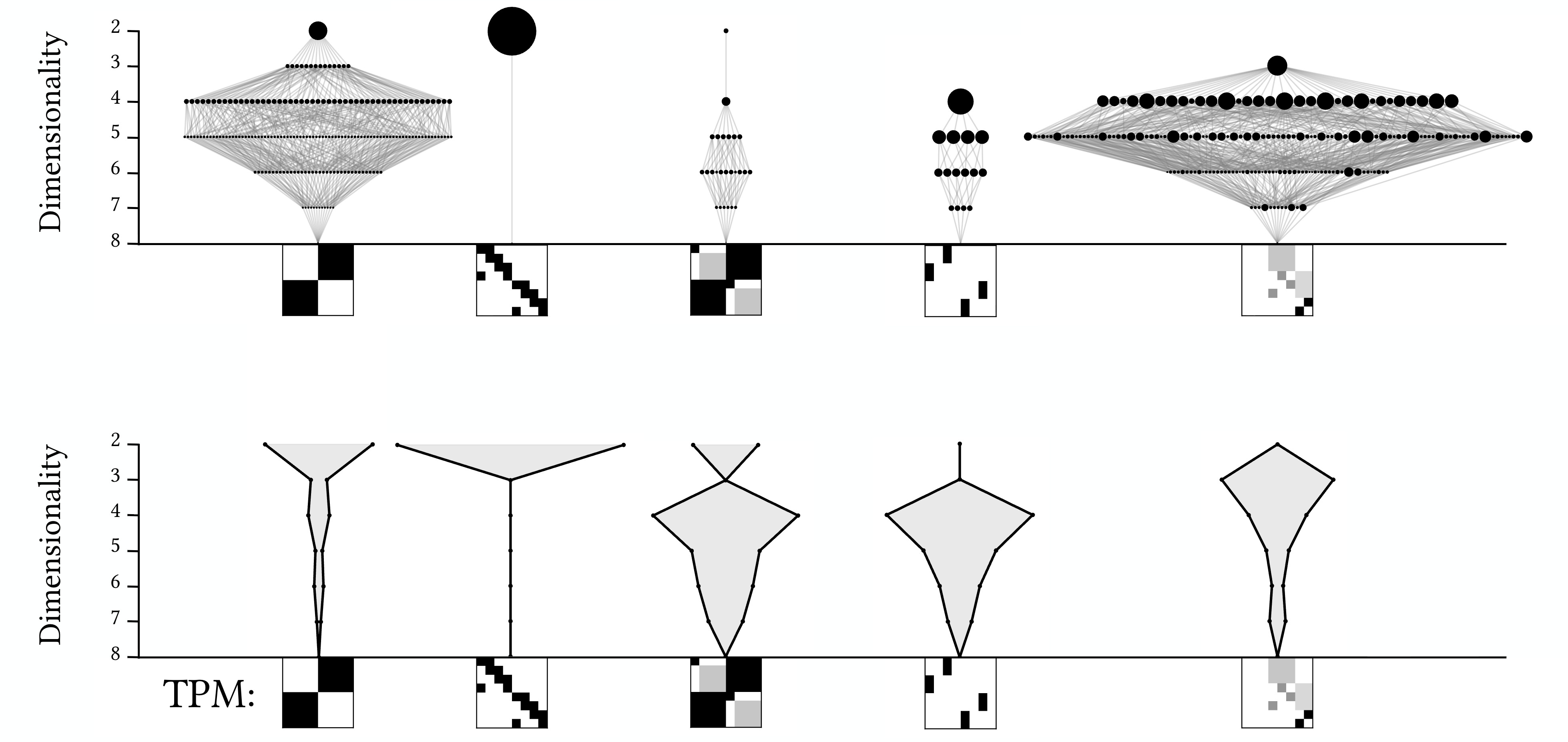
And, they happen to look an awful lot like a landscape of rock formations?
With the ability to dig out the emergent hierarchy (the whole process is much like unearthing the buried causal skeleton of the system) some really interesting questions suddenly pop up.
Like: “What would happen if a system weren’t bottom-heavy, or top-heavy, but if its causal contributions were spread out equally across all its many scales?”
Exactly what we were wondering!
If a system’s emergent hierarchy were evenly spread out, this would indicate that the system has a maximally participating multiscale structure. The whole hierarchy contributes.
In fact, this harkens back to the beginning of the complexity sciences in the 1960s. Even then, one of the central intuitions was that complex systems are complex precisely because they have lots of multiscale structure. E.g., in the classic 1962 paper “The Architecture of Complexity,” field pioneer and Turing Award winner Herbert Simon wrote:
“… complexity takes the form of hierarchy—the complex system being composed of subsystems that, in turn, have their own subsystems, and so on.”
Well, we can now directly ask this about causation: how spread out is the sum of irreducible causal contributions across the different levels of the lattice of scales? The more spread out, the more complex.
To put an official number on this, rather than just eyeballing it, we define the path entropy (as in a path through the lattice from micro→macro). We also define a term to measure how differentiated the irreducible causal contribution values are within a level (called the row negentropy).
At maximal complexity, with causation fully spread out, no one scale would dominate. They’d all be equal. It’d almost be like saying that at the state of maximal emergent complexity the system doesn’t have a scale. That it’s scaleless. That it’s…
Scale-free?
Yes, what a good term: “scale-free.”
Don’t people in network science talk about “scale-freeness” all the time?
Yes, they do.
It’s pretty much one of the most important properties in network science. And it’s linked to criticality and other important properties too.
Yes, it is.
Classically, it means that the network is kind of fractal. If you zoom into a part of it, or out to the whole of it, the shape of the “degree distribution,” as in the overall statistical pattern of connectivity, doesn’t change.
Well, that’s—
But this is different, right? What you’re proposing is literal scale-freeness, not just about degree distribution.
Excuse me, but can I go back to explaining?
Yeah, sure. Go ahead.
Thank you.
Okay, yes, Abel and I define a literal scale-freeness.
First, we can actually grow classically scale-free networks (in the original sense of the term) thanks to Albert-László Barabási and Réka Albert, who proposed a way to generate scale-free networks. It’s appropriately called a Barabási–Albert model, and basically imagine a network is being grown, and then when a new node is added, it enters with a certain degree of preferential attachment, which is controlled by parameter α. When α = 1, the network is canonically scale-free. Varying α results in networks that look like these below (where α, which determines the preferential attachment, starts negative and gets to 1, and then continues on to 4).
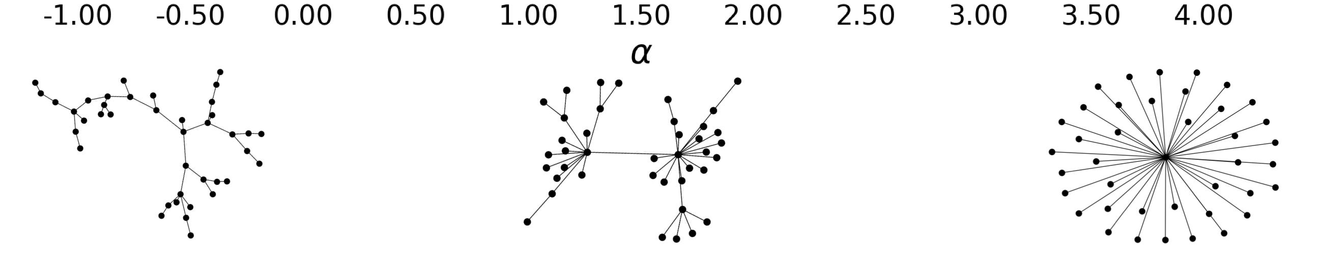
Wait—these are networks. Like dots and arrows. But are they “systems” in the way we defined earlier?
Great question. The answer is that we can interpret them as Markov chains by using their normalized adjacency matrix as TPMs. Basically, we just think of the network as a big state machine. Then it’s as if we’re growing different systems (like different versions of Snakes and Ladders with different rules), and some of these systems correspond to scale-free networks.
So then the emergent complexity should peak somewhere around the regime of scale-freeness, defined by α!
And that’s indeed what we observed. Here’s the row negentropy and the path entropy and, most importantly, their combination, which peaks around α = 1, right when the network is growing in a classically scale-free way.
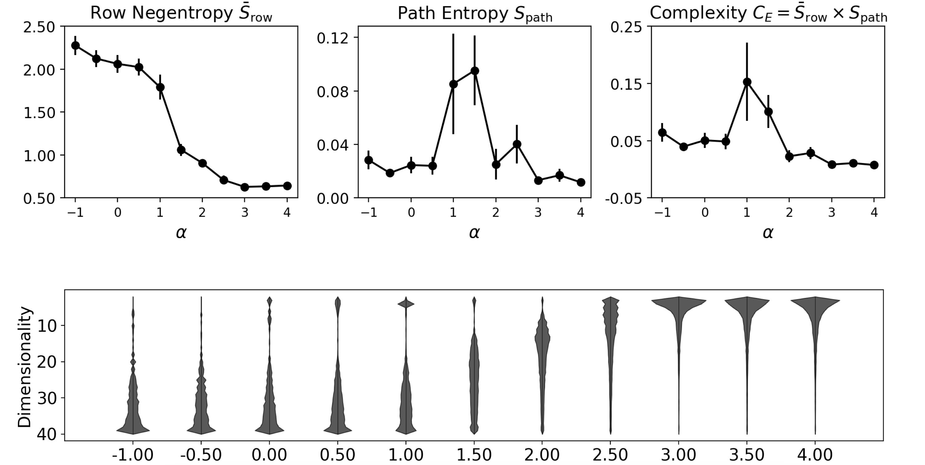
You can see that the causal contributions shift from bottom-heavy to top-heavy, as the networks change due to the different preferential attachment.
Importantly, this doesn’t mean that our measure of emergent complexity is identical to the scale-freeness in network science, just that they’re likely related—a finding that makes perfect sense. The sort of literal scale-freeness we’ve discovered should have overlap, but it should also indicate something more.
Alright, this has been very long, and my brain kind of hurts.
Wait! Don’t go! We’re almost done!
One of the coolest things is that we can design a system to have only a single emergent macroscale. There is no further multiscale structure at all. We call such emergent hierarchies “balloons,” for the obvious reason: it’s as if a single macroscale is hanging up there by its lonesome.
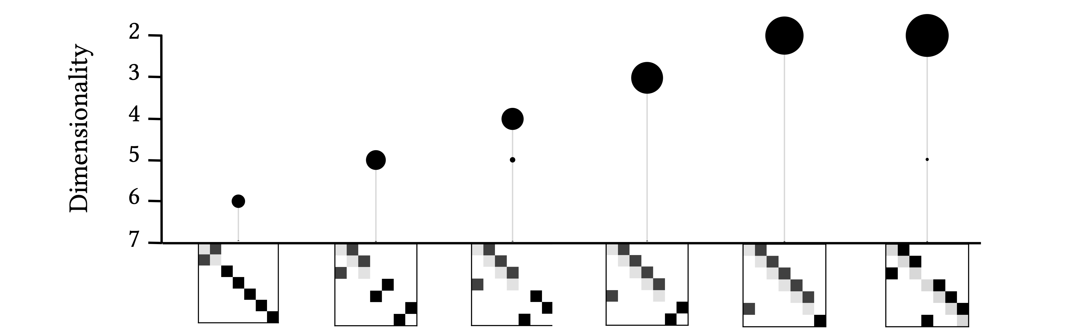
Great! Quick, give me your takeaways.
Right.
Well, ah, I’ll leave all the possible applications for engineering emergence aside here. And the connections to—ahem—free will.
Overall, this experience has made me sympathetic to the finding that “sleep onset is a creative sweet spot” and that targeted dream incubation during hypnagogia probably does work for increasing creativity.
And it’s now my new personal example for why dreams likely combat overfitting (see the Overfitted Brain Hypothesis), explaining why the falling-asleep or early-morning state is primed for creative connections.
But, just to check, do you see it? That some look like rock formations?4
I’m not crazy?
No, you’re not crazy.
Oh, good, thank you.
PLEASE NOTE: this was an overview built for a larger audience, constructed in favor of conceptual understanding. If you want the actual technical terminology and methods, refer to the paper itself, and its companion papers as well. Specifically, “Causal Emergence 2.0” covers more of the conceptual/philosophical background to the theory, while “Consilience in Causation” is about the causal primitives and the details of the causal analysis.
ACKNOWLEDGMENTS: A huge thanks to my co-author, Abel Jansma, for his keen insights (he also made most of these figures, which are taken from the paper). A very special thanks as well to Michael Levin at Tufts University for his continual support.
Why didn’t we notice how to get at multiscale structure from the beginning, back in 2013, in the initial research on causal emergence? Personally, I think it was the result of our biases: Giulio, Larissa, and I had also been used to trying to develop Integrated Information Theory, which specifically has something called the axiom of exclusion. In IIT, you always want to be finding the one dominant spatiotemporal scale of a system (indeed, the three of us introduced methods for this back in 2016). But you can therefore see how we missed something obvious—causal emergence isn’t beholden to the same axioms as IIT, but we originally confined it to a single scale as if it were.
Most other theories of emergence (the majority of which are never shown clearly in simple model systems, by the way, and would fall apart if they did) give back relatively little information. Is something emergent? Yes? Okay, now what? What information does that give? CE 2.0, by finding the emergent hierarchy, gives a ton of extra information about not just the degree, but the kind of emergence, based on how its distributed across the scales. This makes it much more useful and interesting.
The determinism/degeneracy are a bit more complicated than their equations belie. One complication I’m skipping over: to calculate the determinism and degeneracy (and other measures of causation, by the way) you need to specify some sort of prior. This prior (called P(C) in the paper) reflects your intervention distribution, which can also be thought of as the set of counterfactuals you consider as relevant. Usually, it’s best to treat this as a uniform distribution, since this is simple and equivalent to saying “I consider all these counterfactuals as equally viable.”
In the old version of Causal Emergence (1.0), back when it used something called the effective information as the “score” for each TPM, and the theory was based on identifying the single scale with a maximal effective information, the choice of the uniform distribution got criticized as being a necessary component of the effective information. Luckily, this whole debate is side-stepped in Causal Emergence 2.0, because in the new version, which uses related central terms, causal emergence provably crops up in a bunch of measures of causation and across a bunch of choices of P(C). In fact, even when the P(C) of the macroscale is just a coarse-graining of the P(C), and even when P(C) is just the observed (non-interventional) distribution of the microscale, you can still see instances of causal emergence. So the theory is much more robust to background assumptions.
Rock formations shown (in order): Egypt’s “White Desert” and the Bolivian Altiplano.
Bravo! Well done, and beautifully explained. But I confess to some minor annoyance at the end that you defer applying this theory to the question of free will. I hope you can rest from your labors for a bit, then gird your loins and come back to help clarify this controversial issue, which has been muddled in just about every possible way, from the microscale to the macroscale....
Gongshi—spirit stones—along with the stone formations of Joshua tree have been great inspirations for me when studying emergence. Glad to see someone else appreciating this connection